Parametrization of the negative binomial and gamma distribution

Klaus K. Holst

The negative binomial distribution describes the probability of seeing a given number of failtures failures before obtaining $r$ successes in iid Bernoulli trials with probability parameter $p$. More generally, let $X\sim \operatorname{NB}(r, p)$ for real parameters $r>0$, $p\in(0,1)$, then $X$ has distribution given by $$\begin{align*} \mathbb{P}(X=x) = \frac{\Gamma(r+x)}{k!\Gamma(r)}(1-p)^x p^r, x\in\mathbb{N}_0. \end{align*}$$ The stats::rbinom function uses this parametrization, and we have $$\begin{align*} \mathbb{E}X = r(1-p)p^{-1}, \quad \mathbb{V}\!\!\operatorname{ar}(X) = r(1-p)p^{-2}. \end{align*}$$ Further, if $X_1\sim\operatorname{NB}(r_{1}, p)$ and $X_2\sim\operatorname{NB}(r_{2}, p)$ are independent then $X_1+X_2\sim\operatorname{NB}(r_{1}+r_{2}, p)$.

To simulate from a negative binomial distribution with specific mean and variance we can use the carts::rnb function

x <- carts::rnb(1e4, mean = 1, variance = 2)
c(mean(x), var(x))

## [1] 0.98320 1.92371

The negative binomial distribution can also be constructed as a gamma-poisson mixture. We write $Z\sim\Gamma(\alpha, \beta)$ when $Z$ is gamma-distributed with shape $\alpha>0$ and rate parameter $\beta>0$, and the density function is given by $$\begin{align*} f(z) = \frac{\beta^\alpha}{\Gamma(\alpha)}z^{\alpha-1}\exp(-\beta z), \quad z>0. \end{align*}$$

This parametrization leads to $$\begin{align*} \mathbb{E}Z= \alpha\beta^{-1}, \quad \mathbb{V}\!\!\operatorname{ar}(Z) = \alpha\beta^{-2}. \end{align*}$$

We will exploit that the gamma distribution is closed under both convolution and scaling. Let $Z_{1}\sim\Gamma(\alpha_{1}, \beta)$ and $Z_{2}\sim\Gamma(\alpha_{2}, \beta)$ be independent and $\lambda>0$ then $$\begin{align*} Z_1 + Z_2 \sim \Gamma(\alpha_1+\alpha_2, \beta), \quad \lambda Z_1 \sim \Gamma(\alpha_1, \lambda^{-1}\beta). \end{align*}$$

b <- 2
a1 <- 1
a2 <- 3
r <- 0.3
n <- 1e4
## Shape-rate parametrization
z1 <- rgamma(n, a1, b)
z2 <- rgamma(n, a2, b)
## r(z1+z2) ~  gamma(a1+a2, b/r)
plot(density(r * (z1 + z2)))
curve(dgamma(x, a1 + a2, b / r), add = TRUE, col = "red", lty = 2)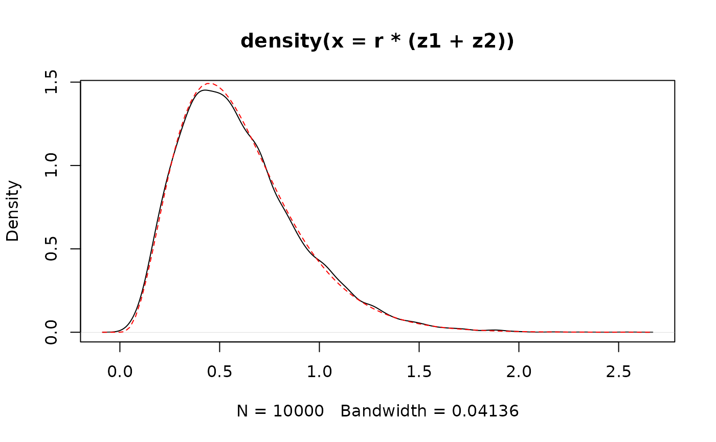

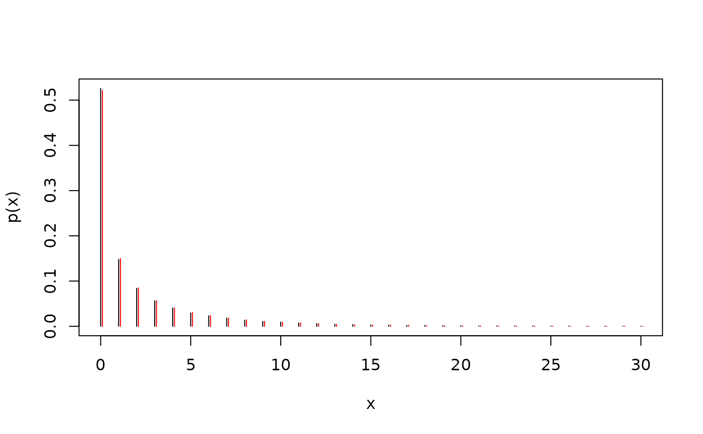
The negative binomial distribution now appears as the gamma-poisson mixture in the following way. If we let $X\mid\lambda\sim\operatorname{Pois}(\lambda)$ with stochastic rate $\lambda\sim\Gamma(\alpha, \beta)$, then $X\sim\operatorname{NB}(\alpha, \beta(1+\beta)^{-1})$.

Consider now $Z\sim\Gamma(\nu, \nu)$, hence $\mathbb{E}Z=1$ and $\mathbb{V}\!\!\operatorname{ar}(Z)=\nu^{-1}$, and let $Y\mid Z\sim\operatorname{Pois}(\lambda_{0}Z)$ for some fixed $\lambda_0>0$, then direct calculations shows that $Y\sim\operatorname{NB}(\nu, \nu(\nu + \lambda_{0})^{-1})$ and $$\begin{align*} \mathbb{E}Y = \lambda_0, \quad \mathbb{V}\!\!\operatorname{ar}(Y) = \lambda_0^2\nu^{-1} + \lambda_0. \end{align*}$$

z <- carts::rnb(1e5,
  mean = 2,
  gamma.variance = 3
)
c(mean(z), var(z))

## [1]  2.00573 14.21768

x <- seq(0, 30)
mf <- function(y, x) sapply(x, function(x) mean(y == x))
plot(x, mf(z, x), type = "h", ylab = "p(x)")
y <- rpois(length(z), 2 * rgamma(length(z), 1 / 3, 1 / 3))
lines(x + 0.1, mf(y, x), type = "h", col = "red")

Bibliography