Getting started

Klaus K. Holst and Benedikt Sommer

Introduction

The carts package is a clinical trial simulation tool for power and sample size estimation. A modular, building-block design allows the simulation of many common clinical trial designs with only a few lines of code. In addition, the package provides a range of estimators for continuous, count and survival endpoints. This vignette introduces the basic functionalities of the carts package and aims to familarize the reader with the package interface. 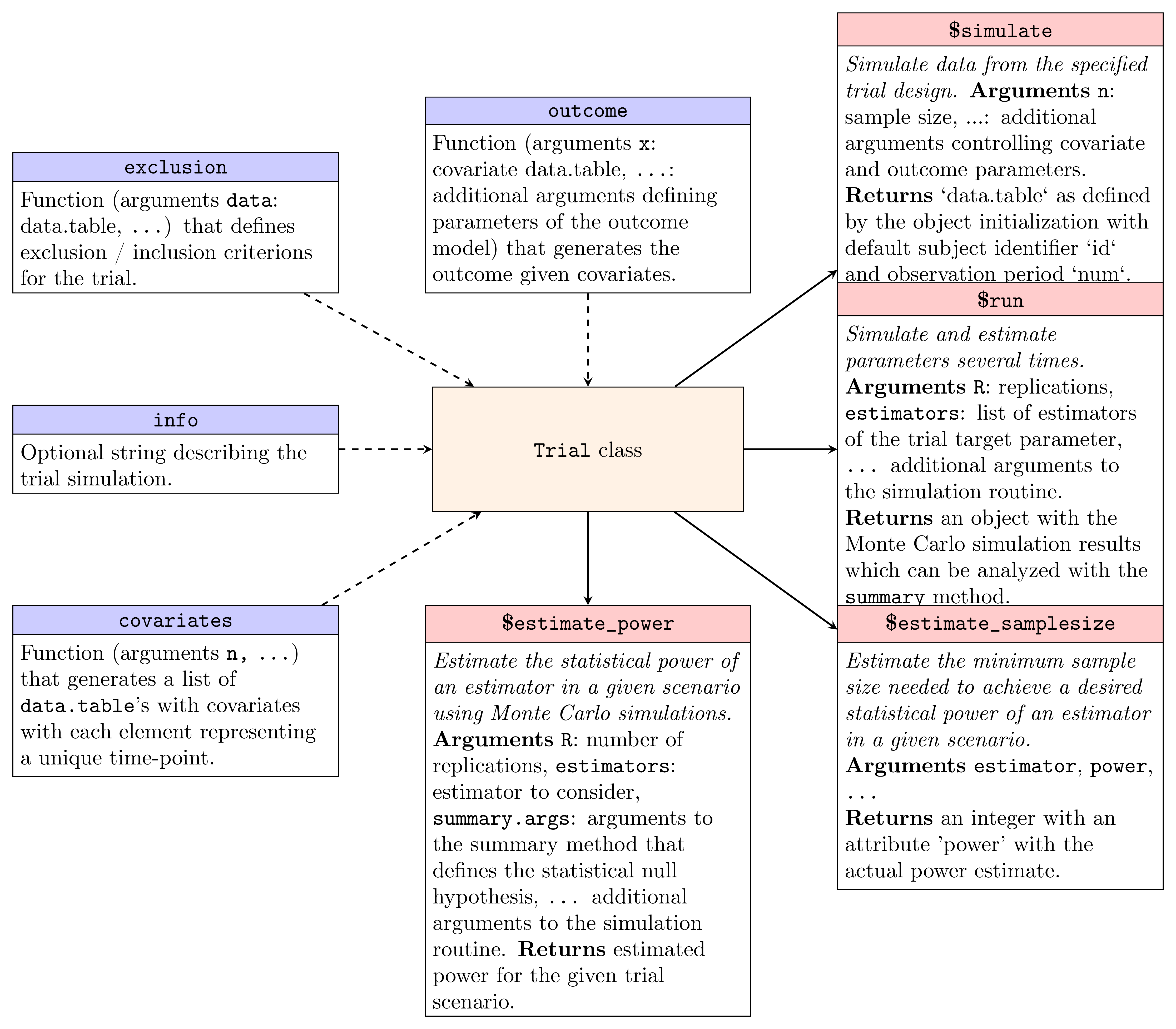The centerpiece of the interface is the R6 reference class Trial, with the constructor and main methods visualized in Figure 1. To this end, we will consider a two-armed parallel trial design to introduce the Trial class and demonstrate how power and sample size estimation are carried out conveniently.

The ‘Trial’ R6 reference class. The blue boxes define the arguments to the constructor, and the red boxes the most important class methods.

Preliminaries

Setting up parallel computations

The carts package is basing its power and sample size estimation on Monte Carlo integration techniques. To deal with the computationally intensive procedures, the package uses extensive parallel computations based on the future package. To enable this, all that needs to be done is to define the desired parallel backend, i.e.

future::plan(future::multicore)

This enables parallelization on all available cores on the current machine. It is equally straight-forward to set up a parallel batch computations on a cluster (see for example future.batchtools).

Progress bars and logging information

As some calculations can be time-consuming we recommend enabling progress-bars, which can be achieved with the following code.

progressr::handlers(global = TRUE)
progressr::handlers(progressr::handler_progress(times = 100))

We refer to the progressr vignette for information on how to customize the progress bar appeareance.

Most output in the carts package is handled by the logger logging utility. We refer to the following article for information on how to alter the logging level and how to change the destination of the log records, which can be useful when running the carts package as batch jobs on a cluster.

Reproducibility

It is sufficient to use a top-level seed for reproducibility of simulations when the future package is used for parallelization on a local machine. Additional care must be taken for distributed computations on a compute cluster.

library("carts")
set.seed(42)

Two-armed parallel design

We will consider a two-armed parallel design where the outcome of interest is $$\begin{align*} Y \mid W, A \sim N(\beta_0 + \beta_w W + \beta_a A, \sigma^2) \end{align*}$$ with treatment variable $A\sim Bernoulli(0.5)$ which is independent of the baseline covariate $W \sim N(0, 1)$.

Trial model

To simulate this trial we first define the random number generators for treatment indicator $A$ and baseline covariate $W$

covariate <- function(n, p.a = 0.5) {
  return(
    data.frame(
    a = rbinom(n, 1, p.a),
    w = rnorm(n)
  )
  )
}

which in the context of carts is a covariate model. The general rule for simulating trial designs with time-invariant outcomes, i.e. outcomes that are only a function of information that is available at baseline/randomization, is that the covariate model is a function with first argument n (sample size) that returns covariate data in tabulated form, either as a data.frame or data.table. Additional parameters of the covariate model can be added after the sample size argument n, being here the treatment probability p.a.

The trial model for this design is completed with the help of outcome_continuous. This built-in function generates continuous outcomes from tabulated baseline covariates, i.e. the output of the covariate model. The default arguments of built-in functions can be updated conveniently with setargs to the desired parameters of the trial. Simulating the trial $$\begin{align*} Y \mid W, A \sim N(10 - 0.5 A - 1.2 W , 1.5) \end{align*}$$ requires to update the default arguments of outcome_continuous as

outcome <- setargs(
  outcome_continuous,
  mean = ~ 1 + a + w,
  par = c(10, -0.5, -1.2), # coef order as defined by the above formula
  sd = 1.5 ** 0.5
)

Finally, we instantiate a model object from the R6 Trial class

trial <- Trial$new(
  covariates = covariate,
  outcome = outcome,
  exclusion = identity, # no exclusion criteria (default)
  info = "Two-armed parallel design" # optional info
)

where, by default, no exclusion model is used.

Trial simulation

Simulating data from the defined model object is done via the simulate method

dd <- trial$simulate(n = 1e4)

The method is a wrapper calling carts:::trial_simulate which combines sampling data from the covariate and outcome model, and the application of the exclusion model in an iterative process. First n subjects are sampled from the covariate model. The sampled tabulated data is then converted into a data.table and passed on to the outcome model. The sampled covariate and outcome data are then passed together as a single data.table to the exclusion model. Thus, the exclusion model allows for removing subjects based on both the covariate and outcome data. If subjects are removed, the remaining subjects are stored and the next iteration begins by sampling from the covariate model. The process repeats until a total of n subjects have been sampled.

Without additional arguments, the method uses the assigned default arguments of the covariate and outcome model to generate the sample.

table(dd$a)
## 
##    0    1 
## 5001 4999

Inspecting the simulated data

head(dd, 2)
##       id     a          w   num        y
##    <num> <int>      <num> <num>    <num>
## 1:     1     1 0.07122244     0 8.165036
## 2:     2     1 0.97029003     0 7.411990

reveals that the package adds subject (id) and period (num) identifiers to the output of the method. This is the default behaviour that provides the functionality to follow subjects across multiple periods in within-subject trial designs.

Updating model parameters

Additional arguments are accepted by the simulate method that allow for simulating from the same trial object while varying model parameters. This circumvents the instantiation of a new model object and provides an elegant way to carry out parameter sensitivity analyses or interactively use a trial model

trial$simulate(n = 1e4, p.a = 0.9)$a |> table()
## 
##    0    1 
## 1017 8983

In fact, most public methods of the Trial class allow passing arguments to the underlying covariate, outcome and exclusion models via the optional argument of the Trial method.

Safeguarding parameter clashes

The simulate method passes all defined model parameters internally to the covariate, outcome and exclusion models. For the given example this means that each of the model component function calls receive p.a = 0.9 as an optional argument. This enables updating shared parameters in all model components with a single value

trial0 <- Trial$new(
  covariates = covariate,
  outcome = function(data, p.a = 0.1) rbinom(nrow(data), 1, p.a)
)
trial0$simulate(1e4)[, list(y = mean(y), a = mean(a))]
##         y      a
##     <num>  <num>
## 1: 0.1009 0.4876
trial0$simulate(1e4, p.a = 1)[, list(y = mean(y), a = mean(a))]
##        y     a
##    <num> <num>
## 1:     1     1

but also opens a pathway to accidentally overwriting default parameters of built-in functions. A simple solution for preventing this is achieved by using functional wrappers. This is shown here for the covariate model, where the default value of p.a cannot be changed dynamically anymore.

trial0 <- Trial$new(
  covariates = function(n) covariate(n),
  outcome = function(data, p.a = 0.1) rbinom(nrow(data), 1, p.a)
)
trial0$simulate(1e4, p.a = 1)[, list(y = mean(y), a = mean(a))]
##        y      a
##    <num>  <num>
## 1:     1 0.4926

Updating default parameters of a trial model

The Trial class also allows to set and update default arguments of covariate, outcome and exclusion models. Another way to utilise built-in functions is therefore to initialize a trial object as

trial <- Trial$new(
  covariates = covariate,
  outcome = outcome_continuous
)

and then set default values for the outcome model with

trial$args_model(
  mean = ~ 1 + a + w,
  par = c(10, -0.5, -1.2)
)

Using the args_model method updates the model.args attribute of the trial object, which are then used internally as the default option to simulate the trial data.

trial$simulate(1e4)[, list(y = mean(y)), by = "a"]
##        a         y
##    <int>     <num>
## 1:     0 10.037275
## 2:     1  9.515117

However, the parameters in trial$model.args are overruled when parameters with matching names are passed to the simulate method.

trial$simulate(1e4, par = c(0, 20, 0))[, list(y = mean(y)), by = "a"]
##        a           y
##    <int>       <num>
## 1:     1 19.99394634
## 2:     0 -0.01365177

Estimators

The carts package provides a range of estimators for various trial designs. All built-in estimators are function generators that return an estimator, which is a function of data (first input argument). To be compatible with the package design, each estimator must return a named vector that includes the estimate (Estimate) and standard errors (“Std.Err”). The returned vector may include additional elements as they not interfere with any internal procedures. A crude (marginal) estimator can be defined by using est_glm, which is a function generator

estimator <- est_glm(
  response = "y", # default value
  treatment = "a" # default value
)
data <- trial$simulate(n = 300)
estimator(data)
##   Estimate Std.Err    2.5%   97.5%  P-value
## a  -0.5394  0.1918 -0.9153 -0.1635 0.004914

Estimators can be assigned to a trial object either during its initialization via the estimators argument of Trial$new or after initialization

trial$estimators(marginal = est_glm()) # using def. args. of est_glm

and all assigned estimators can be retrieved by calling the estimator method

names(trial$estimators())
## [1] "marginal"

or printing the trial object

print(trial)
## ── Trial Object ── 
## 
## Model arguments:  
##  • mean: Class 'formula'  language ~1 + a + w
##  • par:  num [1:3] 10 -0.5 -1.2
## 
## Summary arguments:  
##  • level:  num 0.05
##  • null:  num 0
##  • ni.margin:  NULL
##  • alternative:  chr "!="
##  • reject.function:  NULL
##  • true.value:  NULL
##  • nominal.coverage:  num 0.9
## 
## Covariates:
##  function (n, p.a = 0.5, ...)   
## 
## Outcome:
##  function (data, mean = NULL, par = NULL, sd = 1, het = 0, outcome.name = "y",      remove = c("id", "num"), family = gaussian(), ...)   
## 
## Exclusion:
##  function (x, ...)   
## 
## Estimators:
##   1. marginal 
## ────────────────────

Power estimation

Carrying out power estimations is straightforward once estimators are assigned to the trial model.

trial$estimate_power(
  n = 300, # sample size
  R = 500 # number of Monte Carlo replicates
)
## [1] 0.778

Hypothesis testing

The method uses carts:::summary.runtrials internally to implement the hypothesis test for a given trial design. By default, a two-sided test is carried out for the null hypothesis of no treatment effect with 0.05 signifcance level. The test can be changed via the summary.args argument

trial$estimate_power(n = 300, R = 500,
  summary.args = list(alternative = ">") # one-sided test should
  # have no power as a < 0
)
## [1] 0

Updating model parameters

Arguments to the covariate, outcome and exclusion models can be passed via the optional arguments of the method. The behavior is identical to the one of Trial$simulate. That is, passed arguments overwrite their default values in Trial$model.args.

trial$estimate_power(n = 300, R = 500, p.a = 0.1)
## [1] 0.376

One should note that the current interface does not pass on these optional arguments to estimators. As a consequence, all estimators must be initialized with values assigned to their optional arguments.

Multiple estimators

The default settings of carts is to estimate the power of all estimators that are defined in Trial$estimators.

trial$estimators(adjusted = est_glm(covariates = "w"))
trial$estimate_power(n = 300, R = 500)
## marginal adjusted 
##    0.792    0.992

Sample-size estimations

Last, we estimate the sample size required to attain 90% power for the specified trial model and estimator

# trial$estimate_samplesize(
#   power = 0.9, # default
#   estimator = trial$estimators("adjusted")
# )

The method optimizes the sample size by internally calling the Trial$estimate_power method. Therefore, the behavior for updating model parameters and changing the default settings for the hypothesis test are identical. That is, model parameters are passed as optional arguments or set via the args_model method, and the summary.args argument is used to change the hypothesis test.